UniPlot Objects

UniPlot Documents

A UniPlot document can consist of up to 255 pages. The active page will be displayed on the monitor in the right size ratio. The pink rectangle inside the paper frame is the page margin which can be set in centimeters in the Page Margin dialog box File=>Page Margin.

For each page a tab register with the page name is displayed. To add a new page to the document, choose Edit=>Page=>New Page.

The following figure shows the origin of the page coordinate system:

Paper Size and Paper Orientation can be set in the Page Setup dialog box File=>Page Setup. The paper sizes that are available depend on the capabilities of the printer you have selected. The page can be oriented vertically (portrait) and horizontally (landscape). Page settings will be saved in the document.

The figure above shows the page in portrait orientation with a page margin and a coordinate system which is used to position the objects on the page. The x-axis of the coordinate system points to the right, the y-axis points up. The origin is always in the upper left corner of the page. The coordinates are measured in centimeters.

A page in UniPlot is built from diagrams which are placed on the page. Each diagram can hold datasets and drawing objects. The drawing objects are placed in front of the diagram and the datasets. When you add a new drawing object to a diagram, it is placed in front of all other attached drawing objects. You can change the layering order of diagrams with the One Layer up , One Layer Down , Bring To Front and Send To Back buttons. You can also change the layering order of drawing objects and datasets with these buttons.

To place a drawing object behind the diagrams, it must be added to the background layer.

UniPlot draws the objects in the following order (from back to front):

• Drawing objects in the background
• Diagram rectangle
• Datasets (Fill color, hatch)
• Diagram grid
• Axes with labels and titles
• Datasets (line and marker)
• Drawing objects of the diagram

Document Protection

One way of controlling access to information in UniPlot documents is to set passwords. The Tools=>Protect Document dialog box provide the option to assign a password. When you set either open or modify protection, the password and the contents of the document are not encrypted. If you need higher level of security you should use a different method to protect your documents.

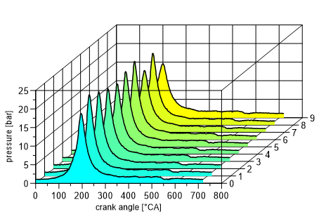
2D Diagram

In UniPlot, a 2D diagram has one x- and one y-axis. The axes are perpendicular to each other. x-values increase to the right and y values increase upwards. If necessary, the axis can be scaled in decreasing order. The y-axis can be placed on the left or right side of the diagram. The x-axis can be placed at the top or the bottom of the diagram. The axes can be hidden if you do not want them to be drawn. They can also be moved parallel to their standard positions.

The following figure shows some examples:

From a single diagram more complex diagrams with several axes can be created. The following picture shows some examples of diagrams with multiple axes.

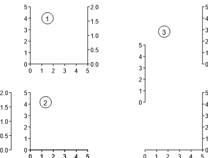
Figure 1 has two y-axes and one x-axis. It is created from two overlapping diagrams. One diagram has the y-axis on the left side and the x-axis at the bottom. The other diagram has its y-axis on the right side and the x-axis is hidden.

Figure 2: y-axes are stacked on the left side of the diagram.

Figure 3 is created from 3 single overlapping diagrams. Only the lower diagram has an x-axis. The x-axis is hidden in the two upper diagrams and linked to the bottom diagram.

Axes of the same type can be linked, therefore they will use the same axis scaling. Linked axes are especially useful for diagrams with multiple y-axes. In figure 3, the x-axes of the upper two diagrams are linked to the x-axis of the bottom diagram. When the scaling of one axis is changed, the linked axes will be rescaled automatically. Only the scaling of an axis is affected by the link. The diagram title, the axis length and other settings of the diagram are not affected through an axis link. To link axes of different diagrams in one page, choose the Diagram Setting dialog box (Diagram=>Diagram Settings). A function written in UniScript is available to create diagrams with multiple y-axes. To execute this function, create an empty page and choose Diagram=>More Diagram Functions to open the following dialog box:

Select Add diagram with multiple y Axes. This function creates a diagram with up to 8 y-axes.

Tip: To move all diagrams on the page to a new location at the same time, select Diagram=>Select All Diagrams and then move the diagrams using the arrow key or the mouse.

Axis scaling and label formats can be adjusted in the Axis Parameters dialog box. The range of the axis can be specified through the Minimum and Maximum values. The Delta parameter specifies the distance between the axis labels. Each label consists of a tick mark and the value of its position.

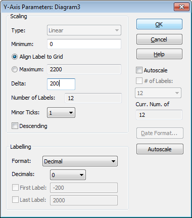
If the axis should start with a value greater than Minimum, click on the First Label check box and type its value into the text box. If the axis should end with a value smaller than Maximum, click on the Last Label check box and type its value into the text box.

Axes are normally scaled in ascending order. You can change this order to descending by selecting the Descending in the Scaling group check box.

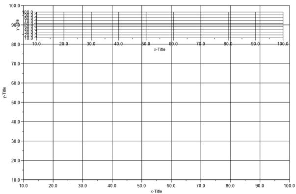
The following figure shows differently scaled axes:

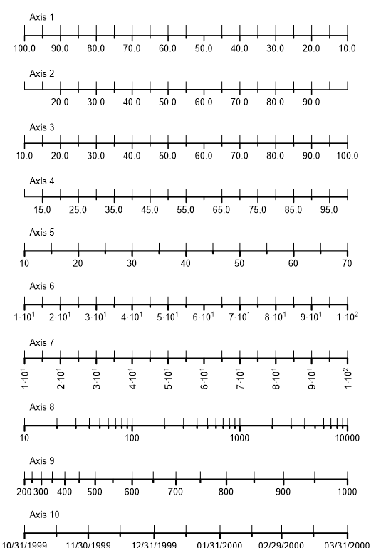
Axis 1 is scaled in descending order.

The minimum parameter for Axis 2 was set to 10 and the maximum parameter was set to 100. The value of the first label was set to 20 and the last label 90.

For Axis 3, the boxes for First Label and Last Label were not checked. In order for the first axis label to begin at 20 even though the axis begins at 10, the text for labels 10 and 100 were deleted from the Label dialog box for this example.

For Axes 5 and 7, labels were created (10 to 70) and days of the week were chosen for the label text in the Axis Label dialog box.

For Axis 6, the exponential format was chosen in the Axis Parameters dialog box.

For Axis 7, the labels were rotated by 90 degrees in the Axis Label dialog box.

For Axis 8, a logarithmic scale from 10 to 10000 was chosen in the Axis Parameters dialog box.

For Axis 9, a square scale from 200 to 10000 was selected.

For Axis 10 a time/date scale for the 10/31/1999 to 03/31/2000 with a step of one month was selected.

Diagrams with multiple axes can be configured as stacked diagrams

Stacked diagrams with multiple y axes

The following figure shows a stacked diagram. The y-axes are arranged on both sides of the grid. The diagram has one x-axis at the bottom.

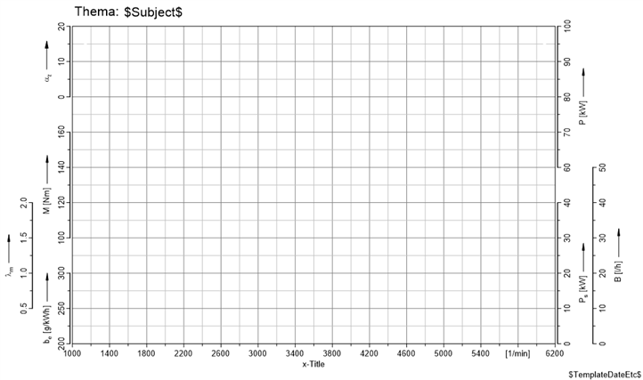
A stacked diagram is created from multiple overlayed diagrams (layers). Each layer displays a y-axis on the left or right side of the diagram. The main advantage of the stacked diagram is that the y-axis scaling will always correspond with the grid lines. Therefore the axis scaling can only be changed in steps so that the axis labels and tick marks correspond with the grid. The y-axis can only be scaled linear.

Every diagram has one layer which displays the grid lines. Normally this layer is placed at the bottom of the Z-order. The grid layer should not contain any datasets. The grid layer displays the x-axis. All other x-axes are hidden and linked to the grid x-axis. The grid layers name should be “grid”.

One page can have multiple stacked diagrams. In this case the layer names are extended by a number, e.g. (Grid1, Grid2,.. etc.).

For a stacked diagram four yellow handles will be displayed in the four corners.

Creating a stacked diagram

• Create at least two diagrams using the button.

• Select both diagrams by holding down the Shift key and clicking on inside the diagram.

  

• Right click on the diagram and choose the command Diagram=>Create Stacked Diagram.

  

• To shift the axis from the left to the right side, grab the axis inside the red bar and move it to the right side. If you hold down the Shift key will dragging the axis will be mirrored.

  Instead of eight handles (blue rectangle at the corners and in the middle of each edge) each layer has only two handles. If you grab the layer inside the handle you can change the axis length. If you grab the diagram at the edge outside the handle you can move the axis up and down.

Features of stacked diagrams

• All layers have the same width and share the same x-axis.
• The grid division is set in the grid layer.
• To select the grid layer click on the x-axis.
• The datasets are clipped at the diagram border if clipping is activated. To activate clipping double-click inside the layer to open the Diagram=>Diagram Settings dialog box.
• One of the layers has the name “grid” or “grid1”, etc.

Changing the diagram size

Modifying the grid division

To edit the grid division click on the x-axis to select the the grid layer. Click the button to open the y-axis parameter dialog box. The parameters Minimum, Maximum and Delta sets the axis scaling, i.e. specify the number of grid lines. If you would like a centimeter grid and the length of the y-axis is 18 centimeters set the values Minimum = 0, Maximum = 18 and Delta = 1.

Adding y-axes

To add another y-axis to the diagram use the and button. To do so click on a y-axis and than click the appropriate button from the toolbar.

If you add a diagram using the button, you can add the diagram by right clicking in the diagram to open the context menu and choosing the command Create Stacked Diagram.

Shifting a y-axis

To shift a y-axis click on the axis. Move the mouse cursor into the red bar and drag the axis to its new position. To edit the axis length, move the mouse into the upper or lower blue handle and edit the axis length. The length can only be changed in the steps of the grid width.

y-Axis Parameter

To align the axis label with the grid the option Align Label to Grid in the Diagram=>X/Y/Z-Axis=>Parameters dialog box must be selected. If the option is selected the Maximum value cannot be set. It will be calculated from the Minimum value, Delta, axis length and the number of grid lines. Since R2012.3 this option can be disabled. The axis can still be part of a stacked diagram, but the axis range can be set freely.

Note

To move the complete stacked diagram click outside of all objects to make sure that no object is selected and then click on the x-axis to select the grid layer. Grab the diagram on the edge of the grid and move it to its new position. You can also use the arrow keys of the keyboard to move the stacked diagram.

3D Diagram

Axes positions for 3D diagrams are selected automatically. Axis elements cannot be clicked with the mouse. To change scaling, labels and the title of an axis, choose the appropriate dialog box from the Diagram menu or select the appropriate button from the toolbar (, , ).

Note

3D diagrams can only be linear scaled. The axis title can only be printed as a single line.

Waterfall Diagram

In a waterfall diagram datasets are stacked into the depth of the diagram.

Data can be imported into a waterfall diagram in the same way as they are imported into a 2D diagram.

Two additional import data functions are available:

• Import of cycles from a single channel: This functions splits perodical data into cycles (File=>More File Functions=>Waterfall-Single Cycle Import).
• Import of multiple channels: This function imports data from multiple channels. One channel can be defined as an x-axis channel. A dataset is created for each selected channel (File=>More File Functions=>Waterfall-Multi Channel Import).

Dataset Objects

With UniPlot, 1D, 2D, 3D (triple) and 3D matrix data can be loaded:

1D Dataset: Points in a 1D dataset are measured equidistantly (e.g. Time signals or crank shaft related signals). The x-value of the first data point and the distance between two points is set in the 2D Curve Configuration dialog box.

2D Dataset: Data points in a 2D dataset set are formed by x/y pairs. The points are added to the dataset in the same order as they are listed in the data file.

3D Dataset (triple): Data points of a 3D dataset which are formed by a x/y/z triple can be irregularly distributed in the x/y plane. To create a 3D dataset, at least 5 data points are necessary. Data points must span a surface above the x/y plane and each point in the plane can have only one z-value.

3D Matrix Dataset: The matrix must have at least 5 columns and 5 rows with z-values. For more details about different format specifications and how you can import a matrix, see Import a Matrix in the UniPlot Reference.

To import data into a diagram, the diagram must be selected. Click inside the diagram frame or choose the diagram’s name from the toolbar.

The data import and the configuration of datasets is covered the chapter Importing Data.

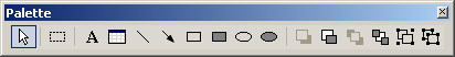
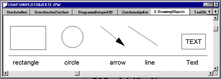
Drawing Objects

UniPlot can create lines, arrows, rectangles, ellipses, text objects and tables. To create an object, choose the appropriate button from the toolbar and drag a rectangle with the mouse where you wish to place the object. The new object will be added to the selected diagram.

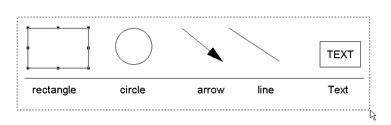
Selecting, Resizing and Moving a Drawing Object

To select a single drawing object, click the object. When the cursor is on the object, the cursor will change to a cross. If the object is transparent, the object can only be selected on one of the object’s lines, not within the object.

Only the drawing objects that are attached to one diagram can be selected. To select more than one object hold down the Shift key and click the drawing objects you want to select.

To cancel a selection, click anywhere in the document outside of the selected drawing object. To cancel the selection of a single object hold down the Shift key and click on the object.

To select several drawing objects from one or more diagrams, select the diagrams the objects are attached to. Then choose the Multi-Select button from the toolbar and drag a rectangle that encloses all of the drawing objects you want to select.

To move a drawing object, position the cursor on the object and drag the object to the new position. To resize the object, position the cursor on an object handle and drag the handle to its new location. The size of a drawing object will be displayed in the status bar in centimeters while the object is dragged.

When you drag the handle of an object, the object is pulled into alignment with the gridline or the nearest intersection of gridlines (Snap-To-Grid effect). To turn off this effect, hold down the Ctrl key while you drag the object. To change the spacing between the gridlines, choose Tools=>Options.

Position and size of a drawing object can also be specified in the object’s dialog box. To open the dialog box, double-click the object.

Tip: To simplify resizing, magnify part of the document. Click the Zoom In button and drag to create a rectangle that encloses the part of the page you wish to enlarge.

The mouse wheel can be used to change the zoom factor. Hold down the Ctrl-key and spin the mouse wheel.

Setting Attributes

To change the object’s settings, double-click the object to open the dialog box. When the cursor is above the object, it will change from a arrow to a cross. Choose your options in the dialog box and click the OK button.

Drawing Order of Objects

The drawing objects will be drawn in the same order in which they were added to the diagram. You can change the layering order within one diagram with the Bring To Front and Send To Back buttons in the toolbar. If you want to send a drawing behind the diagram, or in front of all other diagrams, you have to cut the object out of the diagram and paste it into the background or into the front diagram.

With the Bring To Front and Send To Back buttons you can also change the layering order of the diagrams or change the layering order of the datasets within one diagram. To change their order, only one dataset or one diagram should be selected.

Grouping Drawing Objects

Two or more drawing objects of one diagram can be grouped together to form a single unit. Grouped Objects can be treated as a single object. To group drawing objects, select at least two objects and choose the Group button from the toolbar. To ungroup a Group Object, choose the Ungroup button.

Formula and Latex Text

If the typesetting program Latex is installed you can type in formulas like the following:

See also Edit=>Insert LaTeX Formula.

Text Objects

In the text of an object you can use special characters and the ANSI character sets. Characters or series of characters can be printed in sub- or superscript. Text can contain lines, arrows and symbols.

Image embedded in text

Images can be inserted into text objects, table objects and axes titles.

Example:

@i{n = images\01022012148.jpg h = 1em}

The image must be added to the attachment list.

To insert an image into a table cell, double click a cell. In the following text dialog box click on the Add Image button. The image size can be set using the following parameters:

Display Parameters:

Parameter	Abbreviation	Description
name	n	Image name as displayed in the attachment dialog box.
width	w	Image width.
height	h	Image height.
xoffset	x	Horizontal offset
yoffset	y	Vertical offset
keepratio	k	If set to k=1, the image aspect ratio is kept. For k=0 the height and width can be set separately. k=1 is the default value.

Units for height, width and offset:

Unit	Description
em	Unit is the font height. The font height depends on the selected font.
cm	Unit is centimeter.
mm	Unit is millimeter.
in	Unit is inch.
pc	Unit is pica (1/6 inch).
pt	Unit is point (1/72 inch).
%	Unit is percent of original size (0 to 1000%).

Example:

Value = @i{n=images\ok.png h = 1em}
Image in text @i{n=images\img1.png h = 5cm}

A space is used to separate parameters. A parameter starts with the parameter name or the abbreviation of the name, followed by an equal sign, followed by a value, followed by a unit. The decimal sign is a period.

If the height and width is not specified, the image will be scaled to fit the object size.

If k=1 (default value) is set and the height and width are both specified, the smaller scaling will be used to display the image.

Subscript and superscript

Subscript can be entered by placing the underscore followed by an opening bracket (_{) before the item you want subscripted, and a closing bracket } after it.

Example:

a_{123} will produce

To produce a superscripted character replace the underline with a caret ^ Example: min^{-1} will produce

Bold, Italic, Underline, Strikeout, Color

Within a text object or a cell of a table object, text can be displayed in bold, italic, underline. The font color can also be set. These features are new in R2015.10.

Value	Description
@F{d = 1} or @F{default = 1}	Sets the font the the normal setting: bold = 0 italic = 0 underline = 0 strikeout = 0 color = black.
@F{d = 0} or @F{default = 0}	Has no meaning.
@F{b = 1} or @F{bold = 1}	Switch font to bold.
@F{b = 0} or @F{bold = 0}	Disables bold.
@F{i = 1} or @F{italic = 1}	Switch font to italic.
@F{i = 0} or @F{italic = 0}	Disables italic.
@F{u = 1} or @F{underline = 1}	Switch font to underline.
@F{u = 0} or @F{underline = 0}	Disables underline.
@F{s = 1} or @F{strikeout = 1}	Switch font to strikeout.
@F{s = 0} or @F{strikeout = 0}	Disables strikeout.
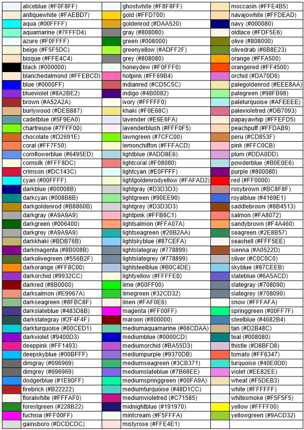
@F{c = red} or @F{color = red}	Sets the font color to red. The color can be specified by its name (see table below) or its RGB value as a hex number starting with #, e. g. red or #ff0000 or #FF0000.

Example:

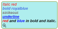
@F{c=red i = 1}Italic red
@F{b = 1 c = royalblue}bold royalblue
@F{s =1 c = grey}strikeout
@F{underline =1 s=0 c = blue}underline@F{default=1}
@F{b=1 i=1 c=red}red @F{c=black}and @F{c=blue}blue@F{c=black} in bold and italic.
@F{b=0 i=1}Q@F{i=0}_{t}

Output:

Color table

Greek letters can be entered by typing a backslash \ before the corresponding latin letter.

Example:

\a \w \l \L will produce

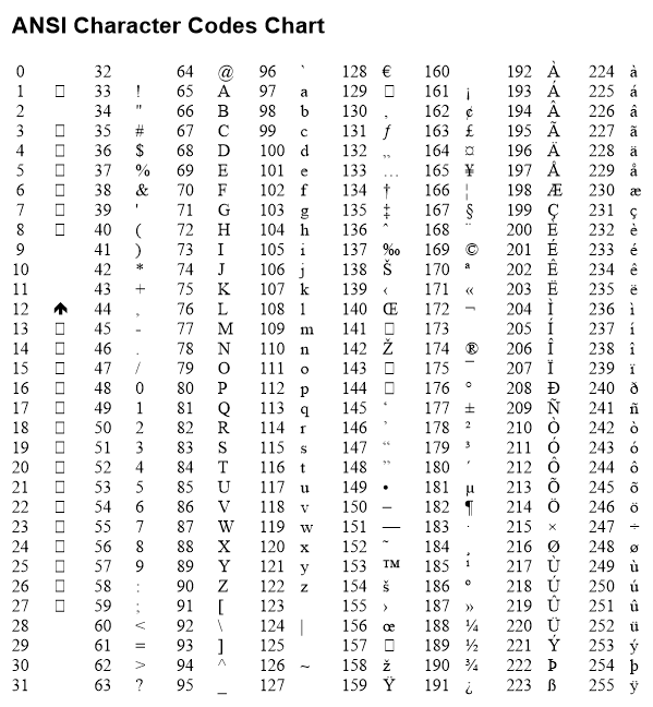
Special characters

Special characters can be produced by using the Character Map program charmap.exe or by holding down the Alt key and typing the decimal value of the character with a leading 0 using the numeric keypad.

Example 1: To create the Copyright-Symbol ©, hold down the Alt key and type 0169 on the numeric keypad.

Example 2: To create the Register character with the symbol font, type in a backslash \, hold down the ALT key and type in the number 0226 on the numeric keypad. The backslash changes the font to the symbol font.

Example 3: To create the Unicode character “LATIN SMALL LETTER M WITH DOT ABOVE”,

• Hold down the Alt key.
• Type the “+”-character (plus) on the numeric keypad.
• Type in the hexadecimal Unicode value, for “m dot” the value 1e41.
• Release the Alt key.

To enable the “Alt+” input mode, add the following key to the Windows registry HKEY_Current_User\Control Panel\Input Method\EnableHexNumpad with the value “1” (REG_SZ). You must restart windows if you created a new key.

Beginning with UniPlot R2012.1 Unicode characters can be inserted into a text using the following code \#xxxx `` where ``xxxx is the 4 digit hexadecimal code of the character. If the code is 4 digits, it must end with a space. The space will be removed. For example 9\#2009 000 will print the value 9000 with a thin space between the 9 and the 000.

For example the “m dot” can be inserted as \#1e41.

Characters with a code greater than 16 bit (e. e. #1D4DD (120029) MATHEMATICAL BOLD SCRIPT CAPITAL N) cannot be specified with 4 hexadecimal digits. Therefore xxxx can be 2 to 6 hexadecimal digits. If 2 or 4 digits are used, the element must end with a space. The space will be removed from the output.

The unicode code can always be set as 6 hexadecimal digits. In this case add 0 to the left. Example: Copyright sign \#0000A9. If 6 digits are used, the ending space is not required.

For most Unicode characters a dot or a double dot does not exists. In this case a combining character can be used, see http://en.wikipedia.org/wiki/Combining_Diacritical_Marks.

For example, a “q dot” can be set as q\#0307 and a “q double dot” can be set as q\#0308.

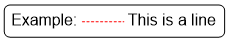
For legends and similar objects, lines, arrows and symbols can be inserted into the text. To add a line to a string in a text object, open the Text Object dialog box and add the following text:

Example: @l{1.1, 1, 3, 255, 0, 0} This is a line

The elements in the example above have the following meaning:

@l{L, S, W, RC, GC, BC}

Value	Meaning
L	Length of the line in centimeters
S	Line style (0 to 5)
W	Line width (thickness) in steps of 0.1 mm
RC, GC, BC	red-, green-, blue-component of the line color (0 to 255)

Available line styles:

Arrows in Text

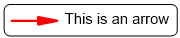
To insert a red arrow into the text, type in the following:

@a{1.2, 0, 5, 255, 0, 0, 1, 0.5, 0.2} This is an arrow

The elements have the following meaning:

@a{L, S, W, RC, GC, BC, P, AL, AW}

Value	Meaning
L	Length of the line in centimeters
S	Line style (0 to 5)
W	Line width (thickness) in steps of 0.1 mm
RC, GC, BC	red-, green-, blue-component of the line color (0 to 255)
P	Arrow position, (0 = left, 1 = right, 2 = left and right)
AL	Arrow length in centimeters
AW	Arrow width in centimeters

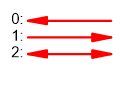
Arrow positions:

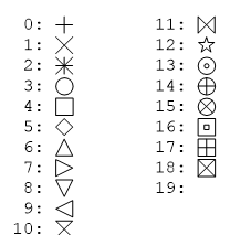
Symbols in Text

To insert a symbol into a text line, type in the following:

@m{0.4,12,1,255,0,255,0,0,0} This is a symbol

The elements have the following meaning:

@m{D, T, W, RF, GF, BF, RL, GL, GL}

Value	Meaning
D	Diameter in centimeters
T	Marker style (0 to 18)
W	Line width (thickness) in steps of 0.1 mm
RF, GF, BF	red-, green-, blue-component of the fill color (0 to 255)
RL, GL, BL	red-, green-, blue-component of the line color (0 to 255)

Available markers:

Spaces in Text

Elements can be moved horizontally with the @s{distance} command. Positive values for distance move the insert position to the right and negative values will move it to the left. The values are entered in centimeters. E.g. @s{-0.5} will move the cursor 0.5 cm to the left.

For example, this command is necessary to create a line element with a centered symbol:

@l{1.2,0,4,0,0,0}@s{-0.7}@m{0.3,15,1,255,255,255,0,0,0}@s{0.5} A Legend String

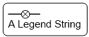
However, you do not have to type in this string. To create a legend for your 1D and 2D datasets, select Diagram=>More Diagram Functions=>Create Legend for 2D Datasets.

For legends and similar objects, rectangles with a hatch filling can be inserted into the text.

Example:

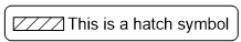
@h{1.2, 2, 2, 0.3} This is a hatch symbol

Syntax:

@h{L, T, B, LD}
@h{L, T, B, LD, RL, GL, BL}
@h{L, T, B, LD, RL, GL, BL, RF, GF, BF}
@h{L, T, B, LD, RL, GL, BL, RF, GF, BF, RK, GK, BK}

The single elements have the following meaning:

Value	Meaning
L	Length of the rectangle (the height is taken from the font).
T	Type (0, 1, 2, 3, …), 0=No hatch
B	Line width (thickness) in steps of 0.1 mm
LD	Hatch line distance in centimeters.
RL, GL, BL	red-, green-, blue-component of the line color (0 to 255). (Default is black (0, 0, 0))
RF, GF, BF	red-, green-, blue-component of the fill color (0 to 255). (Default is transparent)
RK, GK, BK	red-, green-, blue-component of the edge line color (0 to 255). (Default is black (0, 0, 0))

Available hatch styles:

Tabs in Text

The tab character sequence @t{size} can be used to plot text in table form. The number in the braces is the distance of the following text from the left side of the text object in centimeters. In the following example the second column is printed 3 cm and the third column 5 cm from the left edge of the text object.

Field Functions are special codes that instruct UniPlot to insert information into a document. With fields, you can add and automatically update text, page numbers, legends and other information in a document.

Example: The documentname field function inserts the name of the document into a document page. When the document is saved under a new name, the text element is updated.

To insert the field function documentname, create a text element and type @f{documentname} into the element. The result of the field function will be displayed in the document page, e.g. c:\test.ipw.

Text Placeholder

A placeholder is text that begins with a dollar sign, followed by the name, followed by another dollar sign, e.g. $Operator$ is a placeholder for a global attribute. For a channel attribute the channel name followed by a period (.) is placed before the attribute name, e.g. $EngSpd.units$.

Placeholders can be used in text objects, table objects and diagram titles.

To access an attribute from a specific file, add a file alias to the placeholder, e.g. $File1:Operator$. The placeholder $File2:Operator$ would be replaced by the value of the attribute Operator of the second file. Numbering of files aliases starts with 1.

The text must be identical to the attribute name in the NC file. Special characters (. - + $ # ~ ! ^ & %) in the attribute name must replaced by a underscore, for example the attribute speed.units is $speed_units$ as a place holder.

The placeholder can be typed into the text edit control or the name edit control.

Source for the text:

• Edit Object=>Placeholder-Dialog
• File=>Import Data to load global attribute values
• A channel attribute value from an NC file.
• One data point from a channel of a NC file.

Examples for Placeholders:

Placeholder	Description
$Operator$	Global NC-File attribute Operator.
$Origin$	Global NC-File attribute Origin. This attribute contains usally the file name of the original data file.
$Title$	Global attribut with the name Title.
$speed.units$	speed channel attribute units.
$File1:Origin$	Global attribute Origin from the first data file.
$(2)File1:Origin$	The number in parenthesis at the beginning sets the display order in the dialog box.
$File2:speed.units$	speed channel attribute units from the second file.
$speed.1$	First value of channel speed.
$File3:speed.1;%.1lf$	First value of channel speed from file 3. The value will be displayed with one decimal place, see printf.
$File1:speed.-2; %.2lf$	Second last data point of speed displayed with two decimal places.
$speed.i();%.2lf$	Value of a data point. See description below.
$speed.min();%.2lf$	Minimum of channel speed.
$speed.mini();%.2lf$	Index of Minimum of channel speed.
$speed.min_time();%.2lf$	Time of Minimum of channel speed. To define a time channel, use Type = Time Channel as a channel attribute.
$speed.max();%.2lf$	Maximum of channel speed.
$speed.maxi();%.2lf$	Index of Maximum of channel speed.
$speed.max_time();%.2lf$	Time of Maximum of channel speed. To define a time channel, use Type = Time Channel as a channel attribute.
$speed.std();%.2lf$	Standard deviation of channel speed.
$speed.mean();%.2lf$	Mean value of channel speed.

The placeholder $speed.i();%.2lf$ checks, if the global object _g() contains the following member:

_g()._placeholder = [. i = 3]; // Data point 3

If the member variable _placeholder contains a member variable that is identical with the name behind the period (.), in this example i, the value of i is the index of the data point. It can be negative to access the last element.

Usage: Before the function auto_ReplaceTextFromNCFile is invoked a script function sets the the global element:

if (_g().has_key("_placeholder") == FALSE) {
    _g()._placeholder = [.];
}
_g()._placeholder.i = 4;

If the placeholder i does not exists in _g()._placeholder`, the function checks if a function with the name ``_placeholder_i exists (prefix _placeholder_). Example for the max function (placeholder $n_Mot.max();%.2lf$):

def _placeholder_max()
{
   if (_g().has_key("_placeholder") == 0) {
      return "";
   }
   ncid = _g()._placeholder.ncid;
   varid = _g()._placeholder.varid;
   ssFormat = _g()._placeholder.ssFormat;
   rsMax = max(_NC_vargetEx(ncid, varid));
   return nc_val_format(ncid, varid, ssFormat, rsMax, "");
}

To access the channel, the element _g()._placeholder contains the member elements ncid, varid. The member element ssFormat can be used to format the string.

The following functions are already defined: min, max, mean, std. You can add your own functions.

Field Functions

Field functions are especially coded strings in text fields. They can be used to update information in documents automatically. They can be used with table or text drawing objects.

Example: The file name is displayed as a text box in a UniPlot document page. If the document is saved under a new name the field is updated and displays the new name.

Solution: Create a text box and type the following text: @f{documentname}. Instead of the string @f{documentname} the file name is displayed, e.g. c:\test.ipw.

Field Function Syntax

The characters @f{ designate the beginning of a field function, followed by the field function name, followed by a closing brace }. The field function can be followed by a parameter list. The parameters are enclosed by parentheses () and separated by a comma. The comma sign is not a valid parameter character.

After the field function is first evaluated, the field result will be displayed. If you double-click the text element, the field result is placed in braces behind the field function.

Example: @f{date}{11/10/1998}

Fields are automatically updated for some user actions such as. When a document page is opened or closed, a text object is edited or when the data configuration is changed. To force a field function to update its field result, use the shortcut key F9 or choose Edit=>Update Fields.

To enable the text object to adjust its size to the text extension the Automatic Size Update option should be selected (double-click the text object and set the option in the Position and Size dialog page).

Case for field functions is not significant. @f{date} and @f{DATE} are valid field functions.

Inserting Field Functions

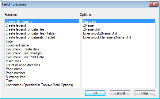
To insert a field function into the active document page choose Diagram=>Insert Field Function to open the following dialog box:

You can also insert a field function manually as follows:

• Click the Draw Text button . Drag to specify the size of the text element.

• Double-click the text element. The text object dialog box will be displayed. Type in the following text: @f{date}
• Choose the OK button.

Writing user-defined Field Functions

You can write your own field functions. The following example shows the definition of the field function @f{pagename}. The name of a field function starts with the prefix __ff_ (2 underscores followed by ff followed by one underscore) (The prefix will be added by UniScript to the field function call). The function name must be specified in small letters. Every field function has 6 parameters. The call parameters which are used in the text element are passed to the field function in the parameter svParameter. The function must return the field result as a scalar string. In case of an error, an empty string ("") should be returned.

User defined field functions should be saved in a file with the extension .ic in the autoload directory. (uniplot/autoload). All ic files in this directory are loaded at startup.

The parameter hText is the handle of the text object which contains the field function. The parameters hLayer, hPage and hDoc are the handles of the parent diagram, parent page and parent document of the text object.

Example:

def __ff_pagename(hDoc, hPage, hLayer, hText, nAction, svParameter)
{
    if (hPage != 0) {
        return PageGetTitle(hPage);
    }
    return "";
}

You can find more field function examples in the UniScript file rs_field.ic.

	Field Functions
@f{3dlegend}	Creates a legend for 3D datasets.
@f{_a}	Displays the text of an alias.
@f{ansi}	Displays an ANSI- or UNICODE character.
@f{area}	Calculates the area for datasets.
@f{channelname}	The field function returns the channelname of the first dataset in the diagram. The field function can be used in a text or table object or in diagram axis title. The text or table object must be assigned to a diagram with datasets.
@f{copytextcolortocurve}	Copy the textcolor of the y-Title text to all 1D and 2D curves. The field function must be located in the y-Title-Text
@f{createdate}	Displays the date when the document was created.
@f{cursor_value}	Displays the x- or y-value of a 2D dataset at the cursor position.
@f{datafilenames}	Writes a list of all used data file names used in the page.
@f{datasetfilter}	Displayes the record filter for the given dataset.
@f{date}	Writes the current date.
@f{documentname}	Writes the document file name.
@f{excel_data}	Displays the specified range of an Excel file in a UniPlot table. The Excel file is linked to the table by the file name. Press F9 to update the UniPlot table in the page.
@f{file}	Writes the contents of a text file (maxium 100 lines).
@f{labeldatapoint}	Labels the data points of the original data with its y value.
@f{labeldataset}	The field functions labels a curve with its legend text, set with XYSetLegendText or the y-channelname.
@f{labelsinglepoint}	Labels a single data point.
@f{lastprintdate}	Displays the date when the document was last printed.
@f{lastsavedate}	Displays the date when the document was last saved.
@f{latex}	Displays a LaTeX Formula in a Text object, axis title of table cell.
@f{legend_table}	Creates a legend table for the data files used in the page or document.
@f{legendchannel}	Creates a legend with the y-channel names of all curves in the diagram.
@f{legendfile}	Creates a legend for all datasets in the parent layer of the text object.
@f{legendstyle}	Creates a legend for a dataset without the legend text.
@f{legendtext}	Displays the legend text of the specified dataset.
@f{legend}	Creates a legend for 1D and 2D datasets.
@f{linkaxisscale}	The function calculates the formula scale * x + offset and displays the result as the new axis scale based on a axis given by the diagram name and axis type (x,y,z).
@f{magnify}	…
@f{marker}	This function can be added to the axis title. It displays the used marker of the first dataset.
@f{ncattfromdata}	Displays the specified attribute from a netCDF file (nc file). The function finds the file name via a specified dataset name.
@f{ncattribute}	Displays a netCDF file attribute (nc file).
@f{ncvaluefromdata}	Displays the value of a data point of a netCDF data file channel. The file name of the netCDF data file will be received via the connected dataset.
@f{pagename}	Displays the page name.
@f{pagenumber}	Displays the page number.
@f{revnum}	Displays the document version number.
@f{scaleaxis}	Creates an axisscale depending on another diagram axis.
@f{summaryinfo}	Displays an item from the summary info dialog File=>Summary Info.
@f{symbol}	Displays a character from the symbol character set.
@f{time}	Writes the current time.
@f{update3dcolorlegendtable}	Color legend of a x/y/z dataset. The field function must be inserted into the name of a table object.
@f{update3dcolorlegend}	Color legend of a x/y/z dataset.
@f{xyinterpol}	Displays the interpolated y-coordinate for a given x-coordinate or the x-coordinate for a given y-coordinate of a 1D or 2D dataset.
@f{xyminmax}	Displays the minimum/maximum coordinates of a dataset.
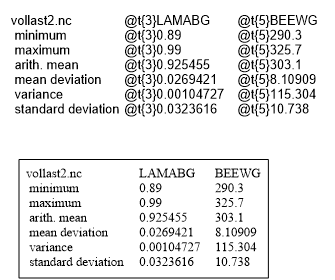
@f{xystatistic}	Displays the following values of a 2D dataset: Minimum, maximum, arith. mean value, mean deviation, variance and standard deviation.
@f{xystatvalue}	Display statistical values for the specified 1D or 2D dataset.
@f{xyvalue}	Displays the x- and y-coordinate of a given 1D or 2D dataset.
@f{xyzstatistic}	Displays statistical information about a 3D map (see example).
@f{xyzstatvalue}	Display statistical values for the specified 3D datasets created from data triples.
@f{xyzvolume}	Calculates the volume, area or the quotient volume/area for a given 3D dataset.

Information/Legend Boxes

The command Diagram=>More Diagram Functions=>Import Page adds the elements of a UniPlot document page to the active page. This function can be used to add standard elements to a page like logos, information legends, etc.

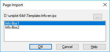
To import a page

• Choose Diagram=>More Diagram Functions=>Import Page.

• The following dialog box will be displayed containing the name of the specified IPW file and the page names of this file.

  

• If the imported page contains a text box, a dialog box will be displayed for text input.

  Example:

  

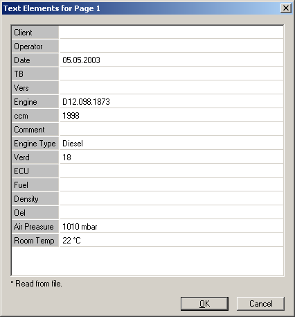
• Type in the information and click OK. The input will be inserted into the text elements

• If you double-click one text element, the text dialog box will be displayed and you can edit the information.

Pages can contain text legends, frames, diagrams, curves, logos, OLE objects etc. Pages should be created separately for portrait and landscape format. The example file \UniPlot\Template\Inofo_e.ipw should not be edited. If you would like to create your own pages or alter the example file, save it under a new name. The example file will be overwritten, if you install a UniPlot update.

To create a new text box

• Choose File=>New. Choose an empty page.

• Create one text object for every text element.

  In the following example, we will create an info box with two elements "Operator" and "Engine". Create four text objects with the text "Operator:", "$(1)Operator$", `` “Engine:”`` and "$(2)Engine$". Then add the rectangle and the horizontal and vertical lines.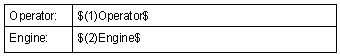

  

• In the next step, we will group all the elements to one object. To do so, select all the drawing objects. Click one object and then choose the Multi-Select button . Drag a rectangle that encloses all drawing objects of this page. Then click the Group button .

• Save the new page (File=>Save As).

• Close the document (File=>Close).

To test the new info box

• Create a new document (File=>New).

• Choose Diagram=>More Diagram Functions=>Import Page.

• In the dialog box that appears choose the button "...". This will open a File Open dialog box. Select the file that contains the new page.

• The file will be opened and the page names will be displayed. Choose the new page name and click OK.

• The page will be imported into the active document page and the following dialog box will be be displayed.

  

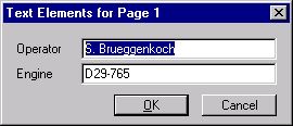
• Type in the text and click OK.

The place-holder text should be enclosed in dollar signs ($) The first dollar sign can be followed by a number enclosed in parentheses () (see example above). The number can be used to set an order for the text dialog. The place-holder with the smallest number will be displayed in the upper left corner of the dialog box.

Place-holders will be replaced by the text. Place-holder text will be copied into the name of the text object. When the text receives a double-click, UniPlot checks if the text object belongs to a grouped object. If this is the case, UniPlot checks if the name of the text object contains dollar signs. If so, the text dialog box will be displayed.

Table Objects

A table object can display text and numbers in columns without using tabulators or blank characters. To create a table click the button from the drawing object toolbar and drag a rectangle with the mouse where you wish to place the table. When you release the mouse button a dialog box will appear in which you can specify the number of columns and rows.

The number of rows and columns is not limited, but if you use the dialog box the number is limited to 50 columns and 50 rows.

To edit the cell text double-click a cell. To navigate to a different cell use the top, bottom, right and left buttons.

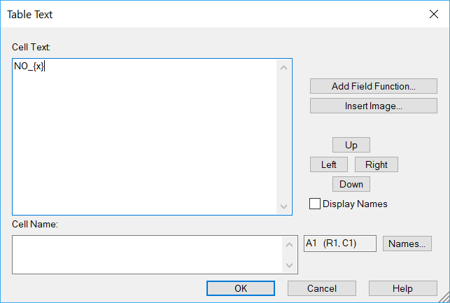
The cell name can contain field functions. Field functions can also be placed in the cell text, e.g the date function @f{date} to display the current date.

Each cell has a name field that can hold a placeholder. The placeholder can be used to be replaced by attributes from a data file. The placeholder value can be edited in a special dialog box.

The cell text can only be printed with one font, i.e. the text can only be displayed in one color with one font size etc. Each cell can use a different font. The text can be rotated in steps of 90 degrees. Cells can be transparent or opaque. The fill color can be set. The cell border line color and width can be specified. Neighboring cells can be merged.

The text alignment can be set.

The font and font color for the cell text can be set using the format toolbar

More configuration options can be set in the dialog box Table Settings. To open the dialog. select one or more cells and right click one of the selected cells. Choose the Configuration command from the context menu. The settings apply to the selected cells.

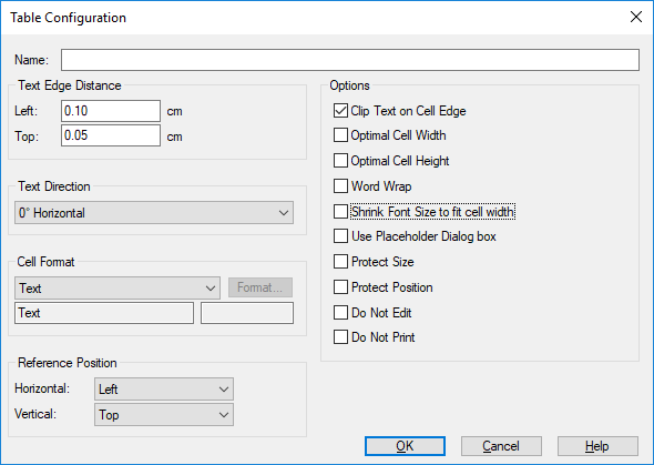
The context menu offers more commands to add or remove columns and rows and copy the contents to the clipboard, etc.

Cell width and height can be edited using the mouse. By holding down the Ctrl key cell width can be set without changing table width.

To drag the table on the page, grab the table on one of the yellow handles.

_id-2051825