Filter Functions for XY datasets
Filter functions are new with UniPlot 4.0. They offer more possibilities to filter and transform the original data of a dataset. A filter, for example, can calculate a cubic spline or remove unwanted points from a curve. They are stored inside the dataset. Filter functions are recalculated when the original data is edited or the datasource of a dataset has changed. The filter functions can be specified for XY datasets (1D or 2D). When a dataset is plotted, the result of the filter function is displayed in the diagram. Optionally, the original data can be plotted as symbols.
For each dataset a list of filter functions can be specified. The first function will use the original data as its input. All other functions will use the output of the previous filter function.
The results of the filter functions are saved in the dataset. If you pass a UniPlot document with filtered datasets to another UniPlot user the result will be displayed correctly, but recalculation of the filter function is only possible if the filter function used in the document are available on the computer.
Filter functions are UniScript functions which can be defined by the user. The following functions can be used as a template for your own filter functions. For more information on writing filter function, move to the bottom of this help topic.
List of filter functions
The source code of the following functions can be found in
script/rs_xy_ffunc.ic.
For the spline, fitspline, pspline and akimaspline functions, the number 0 can be specified for the nPoints parameter. The function then uses a number of interpolation points that depends on the number of original data points n:
n |
nSplinePoints |
|---|---|
0-2 |
100 |
3-5 |
n*100 |
6-19 |
n*50 |
20-99 |
n*10 |
100-999 |
n*5 |
1000-100000 |
n*3 |
>=100000 |
n |
Basic filters
abs - Absolute value
abs()
abs() returns the absolute value.
cumsum - Cumulative sum
cumsum()
Cumulative sum of y-coordinates.
diff - Difference
diff()
Diff calculates the difference between consecutive datapoints.
y(i) = y(i+1)-y(i)
differentiate - Differentiate
differentiate()
Calculates the derivative of the dataset.
mean - Mean value
mean()
Mean value.
min - Minimum value
min()
Calulates the minimum of all given y values.
max - Maximum value
max()
Calulates the maximum of all given y values.
mean - Mean value
mean()
Calulates the mean value of all given y values.
median - Median value
median(nPercent)
Calculates the median of all given y values. Sorts the data in ascending order and picking the middle one if nPercent == 50 percent. The index of the data point can be specified in percent of the number of data points.
Integrate
integrate - Integral
integrate()
Calculates the integral curve using the trapezoidal method.
integrate_cycle - Integral (each cycle)
integrate_cycle(xCycleLength, xCycleStart, nCycle)
Calculates for each cycle the integral curve using the trapezoidal method.
xCycleLength: Length of a cycle in x-coordinates, example: 0.2s or 720 °CA.
xCycleStart: First Point in x-coordinates, example 0s or -360 °CA. xCycleStart is set to x[1] if less than x[1].
nCycle: Number of Cycles. 0 for all cycles.
cycle_value - Integral (cycle/value)
cycle_value(nType, xCycleLength, xCycleStart, nCycle)
Calculates one of the following values for each cycle:
nType can take one of the following value:
1: Mean Value
2: Max Value
3: Min Value
xCycleLength: Length of a cycle in x-coordinates, example: 0.2s or 720 °CA.
xCycleStart: First Point in x-coordinates, example 0s or -360 °CA. xCycleStart is set to x[1] if less than x[1].
nCycle: Number of Cycles. 0 for all cycles.
Scaling
noise - Add Noise
noise(nNoiseInPercent, nMultPoints)
Adds noise to the selected dataset.
scale_x - Scaling-X
scale_x(a,b)
Scales the x-coordinates using x = a*x + b.
scale - Scaling-Y
scale(a,b)
Scales the y-coordinates using y = a*y + b.
correction_factor - Scaling-Y (Correction Factor)
correction_factor(x,y)
Corrects the y-coordinate using a variable correction factor. The filter can be used to correct sensor signal that is known to be deviated on some operating points.

characteristic_curve - Scaling-Y (Characteristic curve)
characteristic_curve(Page:Data Id)
This filter converts the measurement of a sensor into its physical value using a characteristic curve. Ex: voltage into bars for a pressure sensor.
Page: Page of the characteristic curve Data Id: Name of the dataset holding the characteristic curve

Bit
bit - Bit extract and conversion
Extracts a bit form a vector. iBit in the range 1 to 64. The data can be scaled.
bit(iBit, rsScaleFactor, rsScaleOffset)
iBit: Range 1 to 64
Scaling: y = rsScaleFactor * bitValue + rsScaleOffset
If rsScaleFactor is set to 1 and rsScaleOffset is set to 0, the result is in the range 0 to 1.
Clean Data
remove_duplicate_points - Remove duplicate points
remove_duplicate_points()
Removes all duplicate consecutive datapoints with equal x coordinates except the first data point.
remove_original_data_points - Remove original data points
remove_original_data_points()
Removes the original data points from the dataset and sets it to the magic number (x=0.123,y=0.456). This function can be used to save file size. The data exchange will still work.
IMPORTANT: After this function call the filter function cannot be modified until the original data points are reloaded.Example: It can be used in conjunction with the simplify function:
simplify(5);remove_original_data_points()
To shrink the IPW file size, choose File=>Close and Save Compact.
Extract Range
extract - Extract Range (X based)
extract(xmin, xmax)
Extracts data from a curve in the range xmin to xmax. The points at the lower and upper limit are calculated by linear interpolation.
The x-coordinates must be strictly increasing.
see ref:extract_points
extract_points - Extract Range (Point based)
extract_points(imin, imax)
The extract_points function extracts the points from imin to imax.
imin: First point (imin >= 1 and <= Number of points - 2).
imax: Last point. If imax is negative the points are counted starting from the end. Example for a dataset with 17 points:
extract_points(1,22) equivalent to extract_points(1,17)
extract_points(1,-1) equivalent to extract_points(1,17)
extract_points(1,0) equivalent to extract_points(1,17)
extract_points(3,-3) equivalent to extract_points(3,15)
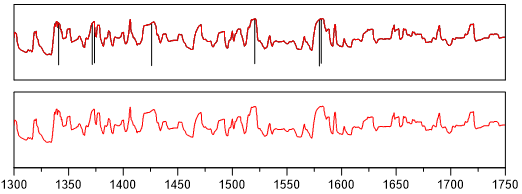
peaks - Extract Range (Peaks)
peaks(Threshold, bAbsolut, Type)
The filter peaks is used to find local maxima and minima in a noisy signal. To use it, create a copy of the signal (Ctrl+C Ctrl+V) and enable markers and the option “Marker for Filtered Data”.
Threshold: Value to detect local extrema
bAbsolut: One of the following values:
0: Threshold value in percent of y data range
1: Threshold value in units of y data
Type: Type is one of the following values.
1: find local maxima (peaks)
2: find local minima (valleys)
3: find local maxima and minima
find - Extract Range (Special)
find(min, max, Axis, Type)
Returns data points in the range min to max. If no data point is found the functions returns the value 0.
Axis is one of the following values:
1: Search x-coordinates
2: Search y-coordinates
Type is one of the followin values:
0: Absolute values (no scaling)
1: Relative values: Values are divided by the maximum before the search (xy / xymax).
2: Relative values: Valurs are scaled to the range 0 to 1: (xy - xymin) / (xymax-xymin).
If Type is 1 or 2 min and max should be set in the range 0 to 1
Example: To find all y-data points in the range 90% of the maximum value, the filter string would be find(0.9, 1.0, 2, 1).
find_plateaus - Detects plateaus
find_plateau(dy_tol, dx_min, dx_max, y_min_threshold, y_max_threshold)
Finds plateaus in the data.
A plateau is found, if the data is inside the tolerance of +- dy_tol. The length in seconds (units as used in ctime) is longer than dx_min and ends at the maximum dx_max or if rvY[i] is greater than the tolerance. Finds only plateaus that are in the range from y_min_threshold to y_max_threshold. A plateau does not contain missing_values.
Each plateau is marked with a constant number, starting with 1, increment 1. The ramps between the plateaus are set to 0.

Frequency
fft_spectrum - FFT: Frequency Spectrum
fft_spectrum(iWindow, Segment_Points)
Calculates the spectrum of the dataset using an FFT.
Segment_Points: 0 (all points), 32, 64, 128, 256, etc.
iWindow is one of the following values:
0: Rectangular Window
1: Hanning Window
2: Hamming Window
3: Welch Window
4: Parzen Window.
5: FlatTop Window
6: Blackmann Window

fft_filter - FFT: Filter
fft_filter(rsFreqCutOffBelow, rsFreqCutOffAbove)
Removes all freqencies from a signal using an FFT. Time must be given in seconds and frequencies are specified in Hz (1/s).
Interpolation
interpol - Interpolation (Linear)
interpol()
interpol(nPoints)
Calculates extra points for a curve through linear interpolation.
nPoints: Number of points of the new curve or a list of x-coordinates separated by a comma.
interpol2 - Interpolation (Linear-min/max/delta)
interpol2(xmin, xmax, xdelta)
Calculates extra points for a curve from xmin to xmax with an increment of xdelta through linear interpolation.
The dataset must be monoton. If xmin or xmax is out of x-range the range will be corrected. The function cannot perform an extrapolation.
interpol_cosine - Interpolation (Cosine)
interpol_cosine(nPoints)
Calculates extra points for a curve through cosine interpolation.
nPoints: Number of points of the new curve or a list of x-coordinates separated by a comma.
Smooth
smooth - Smooth (moving average)
smooth()
smooth(nNeighbor)
Smooth a dataset with the moving average.
The optional parameter nNeighbor specifies the number of points used
the moving average. nNeighbor specifies the window width. The window width is
2 * nNeighbor + 1.
The If the parameter is not specified, it is set to 10.
With the help of the optional parameter PeakFilterFactor peaks can be
keept in the filtered signal. If set to 0 all peaks are smoothed.
This is how the Peak-Filter works:
The smooth function will be applied on the original data.
The difference between the original and the filtered data is calculated.
The difference is multiplied with PeakFilterFactor (Range 0 to 1) = dy.
All points of the original data with a difference greater than dy are inserted into the filtered signal.
smooth_median - Smooth (moving median)
smooth_median(nNeighbor)
Running median. nNeighbor is the window size of the moving window in the range 3 to 1025. Even numbers will be rounded up to the next odd number. For each window the middle value found is used. The filter can be used to reduce random noise and spikes. (see moving_median).
Example: smooth_median(5)
5 consecutive points are sorted ascending and the third point is used. For a window size of 5, the first 2 point and the last 2 points are not altered.
given: [5, 7, 6, 4, 27, 8, 4, 5]
result: [5, 7, 6, 7, 6, 8, 4, 5]
Example:
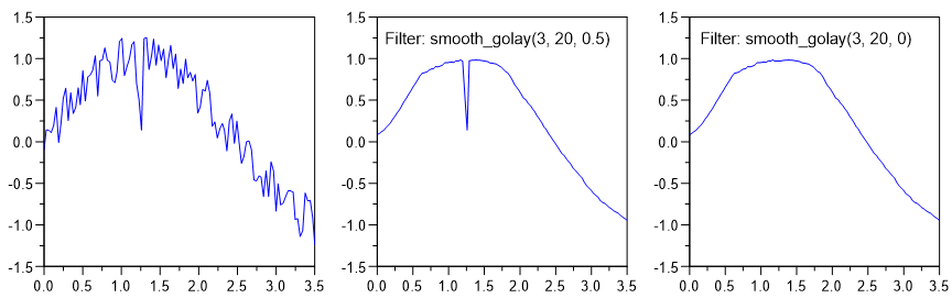
smooth_golay - Smooth (Savitzky-Golay filter)
smooth_golay(nPolynomialOrder, nWindowSize)
smooth_golay(nPolynomialOrder, nWindowSize, PeakFilterFactor)
A better procedure than simply averaging points is to perform a least squares fit of a small set of consecutive data points to a polynomial and take the calculated central point of the fitted polynomial curve as the new smoothed data point.
The smoothing effect of the Savitzky-Golay algorithm is not so aggressive as in the case of the moving average and the loss and/or distortion of vital information is comparatively limited.
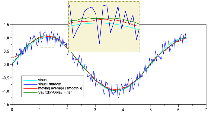
Peak-Filter. The method is identical to the smooth-funcition.
smooth_time - Smooth (with Time Window)
smooth_time(rsTimeWindow)
Smoothing with moving average. A point p of the polygon is calculated by computing the average of p and 2*n neighbor points.
Mean_i = sum(i-n .. i+n) / (2*n+1)
rsTimeWindow: rsTimeWindow specifies a window of the given size in the untis of the x channel. The neighbor points n is the number of points inside the window
Polynom Fit
spline - Spline (Cubic)
spline()
spline(nPoints)
Calculates a cubic spline that will cross all datapoints.
nPoints: Number of spline points (Default = 1000). The number must be in the range of 10 to 100000.
fitspline - Spline (fitspline)
fit_spline()
fit_spline(smoothfactor)
fit_spline(smoothfactor, nPoints)
The Fit Spline function fits a smoothing spline using a smoothing parameter you specify.
smoothfactor: A value of 0 meas no smoothing (i.e. the spline will cross all original data points) and a value greater as 0 will create a smooting spline.
nPoints: Number of points in the range 10 to 100000.
akimaspline - Spline (Akima)
akimaspline()
akimaspline(nPoints)
Akima spline interpolation better copes with discontinuities in a time series than normal cubic splines. The interpolation approximates a manually drawn curve better than the ordinary splines, but the second derivation is not continuous.
nPoints: Number of spline points in the range 10 to 100000.
rspline - Spline (Rational)
rspline(nPoints, TensionFactor)
Rational spline interpolation better copes with discontinuities in a time series than normal cubic splines.
nPoints: Number of spline points in the range 10 to 100000.
TensionFactor: parameter to straighten the curve (0 to 100).
pspline - Spline (Parameter Spline)
pspline(f, nPoints)
If f is nearly zero (e.g. .001) the resulting curve is approximately a cubic spline. if f is large (e.g. 50) the resulting curve is nearly a polygonal line.
f: Tension Factor.
nPoints: Number of Points (3 to 100000). nPoints = 0: automatically creates number of points.
oldspline - Spline (old version)
oldspline()
Calculates a cubic spline that intersects all data points. This function exists
for compatibility reasons with UniPlot 3.x. Use the function spline(0)
instead.
polyfit - Polynomfit
polyfit()
polyfit(polynomOrder)
polyfit(polynomOrder, nPoints, nInfoText)
polyfit(polynomOrder, nPoints, nInfoText, xMin, xMax)
Polynomial curve fitting.
polyfit finds the coefficients of a polynomial p(x) of degree n that fits the data, p(x(i)) to y(i), in a least squares sense. Creates a fit polynom of degree 0 to 9. The polynomial of degree 1 is the regression line.
polynomOrder: Order of polynom (default = 1). 1 creates a straight line (linear regression).
nPoints: Number of points of the fitting curve (default = 1000). The number of points should be in the range 2 to 100000.
nInfoText:
0 = no text.
1 = Polynom parameter.
2 = Polynom parameter and R2(coefficient of determination).
xMin: Start value, can be smaller than the first x-data value. If set to 1e10, the x-minimum of the dataset will be used.
xMax: End value, can be larger than the last x-data value. If set to 1e10, the x-maximum of the dataset will be used.
polyfitzero - Polynomfit (Y-intercept at 0)
polyfitzero()
polyfitzero(polynomOrder)
polyfitzero(polynomOrder, nPoints, nInfoText)
Fit polynomial to data, forcing y-intercept to zero. Creates a smoothing polynom of the order 0 to 9.
polynomOrder = 1 creates a straight line (linear regression).
nPoints: Number of data points (Default = 1000)
nInfoText:
0 = no text
1 = Polynom parameter
2 = Polynom parameter and R2 (coefficient of determination)
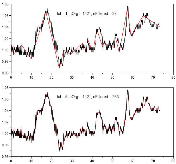
simplify - Simplify
simplify()
simplify(nTolerance)
Polyline simplification using the Douglas-Peucker algorithm.
nTolerance: Specified the maximum distance between the original curve and the simplified curve. A value of 1 sets a tolerance of 10%. The values 2,3,4,5, etc. always divide the tolerance by 2. Therfore a value of 4 is a tolerance of 1.25%. A value of 30 sets a tolerance of almost 0% Default value is 5.
Advanced
boundary - Data Boundary
boundary()
boundary(type)
boundary(type, width)
Calculates the upper, lowert or upper and lower hull curve.
type
0 - upper hull (Default value = 0).
1 - lower hull.
2 - upper and lower hull.
width: Class width in percent (Default value = 5%).
center - Center of a cloud of points
center()
Center of a cloud of points. Calculates the average of the x and y coordinates. Displays a marker at the center.
Important: Enable Marker for filtered data!
convex_hull - Convex Hull
convex_hull()
Calculates the convex hull of the dataset.
event_duration - Event Duration
event_duration()
Computes the duration of all the high events of a boolean signal and outputs a dataset where:
X: start of the event
Y: duration of the event
The example below shows a typical usage of this filter.
Apply a find filter to a curve to target specific events
min = 0
max = 0.7
Axis = 2
Type = 3 (1 when min/max condition is met and 0 otherwise)
Apply an event_duration filter to compute the duration of each high event.
Right-Click => Text Object => 2D-Table to get a table out of the dataset.
Add conditional formatting to the table to quickly highlight needed information.

histogram - Histogram
histogram(Type, ClassMin, ClassMax, ClassWidth)
Calculates a histogram.
If ClassMin=0 and ClassMax=0 then ClassWidth is number of bins in the y-data range.
ClassMin and ClassMax, if not auto, are the lower left value of respectively the minumum of the 1st class and the maximum of the last class (not the center!).
Type can be one of the following values:
1: Absolute
2: Percent
3: cumulativ (‘more than’)
4: cumulativ in percent (‘more than’)
5: cumulativ (‘less than’)
6: cumulativ in percent(‘less than’)

see histogram
range_counting - Range Counting (DIN 45667)
range_counting(rsThreshold)
Range counting is standardized in DIN 45667.
DIN 45667: Classification methods for evaluation of random vibrations. The spans between successive extreme values are determined. The sorted spans are plotted.
Add the histogram filter to create a histogram from the result.
Parameters:
rsThreshold: Minimum span, smaller spans will be ignored
nType: 1 All amplitudes
nType: 2 Only positive spans
nType: 3 Only negative spans

set_to_zero - Set to 0 above threshold
set_to_zero(rsThreshold)
Sets a curve to 0 if a threshold is crossed.
sort - Sort
sort()
Sorts the data in ascending order based on the x coordinate.
step - Step
step()
step(nType)
Calculates a cityscape or skyline curve
nType can take one of the following value:
0 - Curve starts horizontal.
1 - Curve starts vertical (Default value = 1).
to1d - x/y => t/y (1D)
to1d()
Converts an x/y data set into a t/y data set. The x-coordinates are distributed evenly over the entire x-coordinate range.
Writing Filter Functions
Below is an example on how to write filter functions
def _xy_filter_func_scale(hData, a, b)
{
    if (nargsin() == 1) {
        _a = 1;
        _b = 0;
    } else if (nargsin() == 2) {
        _a = a;
        _b = 0;
    } else if (nargsin() == 3) {
        _a = a;
        _b = b;
    }
    xy = XYGetData(hData);
    x = xy[;1];
    y = xy[;2];
    y = _a * y + _b;
    return XYSetData(hData, x, y, TRUE);  // Don't forget the TRUE!
}
def _xy_filter_info_scale()
{
    svInfo = ["Y-Skalierung";
              "scale(a,b)\n\nScales the y-coordinates with the help" + ....
              "of the equation y = a*y + b";
              "";
              "2";
              "Factor a:1:-1e9:1e9";
              "Offset b:0:-1e9:1e9"];
    return svInfo;
}
To define a new filter function, two functions need to be written. One function
calculates the data, the other provides information to the user interface. In the
example above these two functions are _xy_filter_func_scale and
_xy_filter_info_scale.
The filter function names begin with _xy_filter_func_, followed by the
functions user namen in this case scale.
The functions can be saved in a file with en extension .ic in UniPlot’s
autoload directory. When UniPlot is started the functions will be loaded
automatically.
The info function returns a string vector with at least 4 elements:
Element |
Meaning |
|---|---|
svInfo[1] |
Function name. |
svInfo[2] |
Info text shown in the Help windows. If the text is long it can be spaced over various lines as in the example. The rows will be linked with |
svInfo[3] |
Not used. Must be an empty string (“”). |
svInfo[4] |
Number of parameters “0” to “8” |
svInfo[5,6,..] |
(Optional) Parameter name, default value and range separated by a colon (:). |
The func function makes the calculation. The dataset handle will always be the first parameter. Data from the dataset can be accessed using the handle (XYGetData). The results will be written with the XYSetData function. The other parameters are option and must match the definition in the info function.
History
Version |
Description |
|---|---|
R2026.3 |
find_plateaus |
R2024.4 |
xy_filter_event_duration correction |
R2024.3 |
|
R2022.2 |
id-1866448