A Simple Example

The following example will help familiarize you with some of UniPlot’s functions.

Task: To produce an isoline diagram and a 2D diagram with a Full Load Line (Wide Open Throttle curve or WOT).

Creating a Document

In the first step, we will create a new document with two diagrams. Click the New button in the toolbar or choose File=>New.

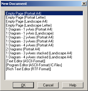
In the New Document dialog box, select the 2 Diagrams (Portrait) option and click the OK button or just double-click the item.

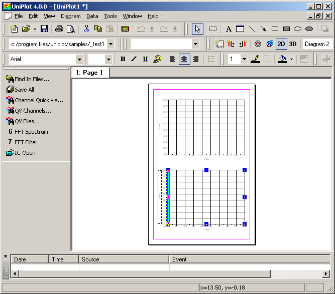
A new window with a portrait oriented page and two diagrams will be created. The page and pink margins will help you to position the diagrams and the drawing objects. These elements will not be plotted on the printer. To change page margins, choose File=>Page Margin. To change the paper size and orientation, choose File=>Page Setup. The options in the Page Setup dialog box depend on the capabilities of the selected printer.

You can change the Page Setup at any time. However, the position of drawing objects and diagrams will not be adjusted automatically to the new settings.

Importing Data into a Diagram

In this step we will import a 3D dataset.

A 3D dataset can either be created from x, y, z data that is irregularly distributed in the x/y plane or from data that is already in a matrix form. In this example, we will create the dataset from the fuel consumption data of an engine versus speed and torque with an irregular distribution.

Import Options: Before we import the data, we will choose File=>Import Options. In this dialog box, you can select column separators for Text files. The columns can be separated by blank and tab characters, one comma, one semicolon or one tab character. For text files, the decimal separator can appear as a point (".") or a comma (",").

If the data columns have names above the data points, the name can be loaded and used to label the axis and the datasets.

Example data files are located in the uniplot\samples directory. To see how the data files are formatted, load one data file into an editor. Choose File=>Open and load the map2.asc file. The data columns in this file are separated by blanks and the decimal separator is a point. The names of the columns appear 2 rows before the first data row. Before loading the data into a diagram you should close the editor with the File=>Close function.

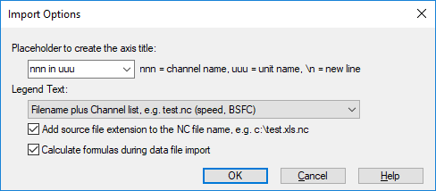
For the map2.asc data file, information should be entered into the File=>Import Options box as shown below.

After you have set the options, choose File=>Import Data. In the dialog box, select the map2.asc file from the uniplot\samples directory. The file will be opened and converted into a netCDF file. The name of the netCDF file will remain the same but the extension will be changed to .nc.

If a file with the same name already exists, a message box appears. The existing file can be written over or the new file can be saved under a different name.

If the text file was successfully converted to a netCDF file, the Import dialog box will appear.

The list of variables X, Y, Z shows the converted data columns. Only the columns with values will be converted. Any other columns, such as time or date columns, will be skipped. The only exception is the definition of the Full Load Line (WOT) for 3D datasets.

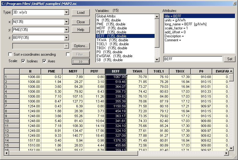
To open it to its full size click the button. The key word "double" in front of the variables means that the data points of the variable are float numbers with double precision (8 Bytes). The number in brackets behind the variable is the number of data points.

The data points of the selected variable are listed in the left list box of the dialog box. To edit a value in the list box, select the data point in order to copy the value into the text field. To set the data point to a new value, choose the Set button.

The attributes of each variable are displayed in the attributes list box underneath the variables list box.

The variable Global Attribs hasn’t any data points. This variable has only attributes. The Range attribute has a special meaning for 1D and 2D datasets. It consists of two values separated by a comma. The first value is the index of the data point where the import should start and the second value is the number of data points that will be imported. Default is "1, Total Number of Points".

Caution: Any changes to data points and attributes will be saved immediately in the netCDF data file.

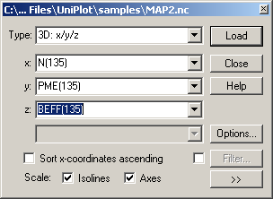
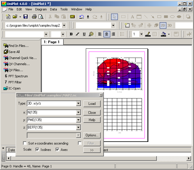
In the Reading Instructions dialog group, you can select the type of the dataset and the data columns you want to import. To import a 3D dataset, click the 3D radio button. The isoline and axes check boxes should be selected in order to scale the axes and isolines automatically.

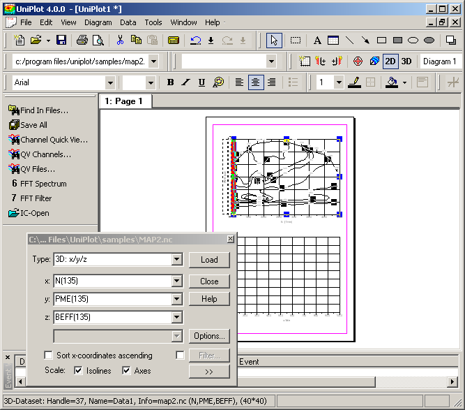
Before importing a dataset, we need to select the diagram the dataset should be assigned to. Click inside of the top diagram. The name of the selected diagram will be displayed in the toolbar.

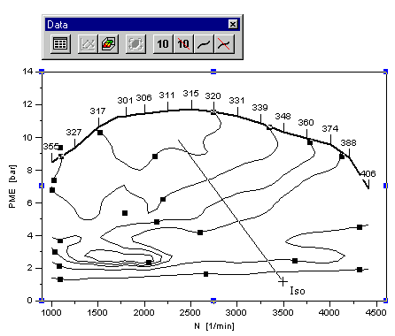
Now we are ready to import the 3D dataset to create a fuel consumption map. Assign the variable N to the x-axis, the variable PME to the y-axis and the variable BEFF to the z-axis. When you have set the variables, select the Load button to import the data into the selected diagram.

During the import, data points will be read from the file and saved in a dataset object. An equidistant matrix with z-values will be computed from the imported data points. In the next step, isolines will be calculated from the interpolated matrix. As well as the original data and the interpolated matrix, other information will be stored in the dataset object i.e. the isoline values, fill colors, label fonts, the dataset hull, label format, etc. This information will be initialized with default values during the creation of the dataset. Default values for dataset objects, diagrams and drawing objects can be set in the Tools menu.

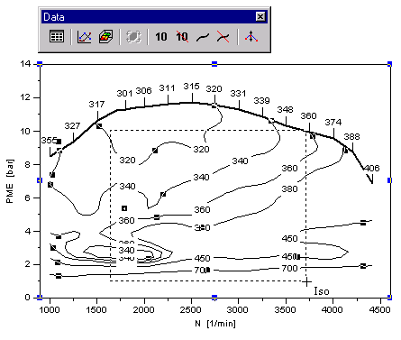
Isolines and their labels will be created automatically. In the next step, we will change their distribution and the position of the labels.

Editing Isolines

Parts of the document can be magnified using the Zoom function to enable easy editing of isolines. Choose the Zoom In button and drag a rectangle around the part of the diagram to be enlarged. The Zoom Out button will reduce the document size to fit into the window. If you click the Zoom Out button repeatedly, you can switch between the full size window, 50% of the window size and the original size.

In the first step, we will delete the isoline labels. Choose the Delete Label button with the crossed out 10. The mouse cursor will change to a cross with the label Iso. Position the cross cursor in the upper left corner of the diagram and drag a rectangle that encloses all of the isoline labels. The labels inside the rectangle will be removed from the map.

Any mistakes that might have been made inserting and deleting isolines and their labels can be eliminated using the Replot button from the toolbar or press Ctrl+R.

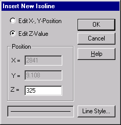
Next, we will add new isolines to the map. Choose the button from the toolbar. Click a point on the map with the cursor. You can only insert lines inside the data hull of the map. If you click outside of the map, UniPlot will switch back to the Selection mode and the cross cursor will return to the shape of an arrow cursor .

If you click inside of the map, a dialog box with the x, y, z coordinates of that point will appear. Choose OK to insert the line into the map.

To label the isolines, choose the Insert Label button from the toolbar. Draw a line by holding down the left mouse button and dragging the mouse. The line must cross at least one isoline. A label will appear at each point where the line intersects an isoline. To insert a single label, click a point on the isoline where you want the label to appear.

The labels on the Full Load Line (WOT) cannot be edited in the same way. Full load line label editing is covered in the chapter “Definition of the Full Load Line” .

To delete an isoline, choose the button with the crossed out isoline and click the isoline which you want to remove. An isoline can consist of more than one line segment of the same value. This function deletes all single line segments of the same value and their labels.

Click outside of the map to switch back to the Selection mode. The cursor will change back to an arrow.

3D Dataset Configuration

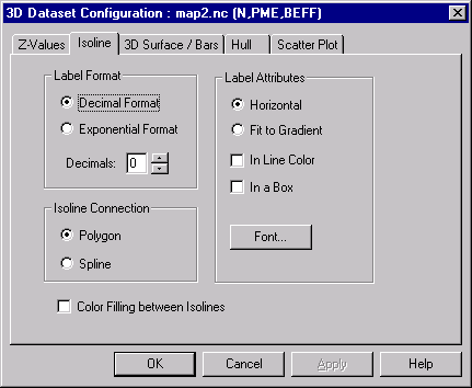
Next we will define a color gradient for the map. Double-click one isoline to open the 3D Dataset Configuration dialog box and the select the Isoline tab. Select the Color Filling between the Isolines check box. In this dialog page you can also specify the format and alignment of the isoline labels.

To modify the default color gradient, select the Z-Values tab. In the list box, the iso values of the map, the fill colors and the line style for the isolines are displayed. The values are sorted in increasing order. Fill color is used to fill the area between the value that is displayed beside the fill color and the next bigger value. To be able to define a fill color for even the smallest value, the value min has been inserted at the beginning of the list.

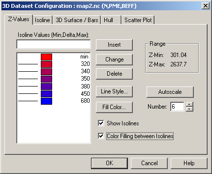
When you select a value from the list, it will be transferred to the edit field above the list. Edit the value and then click the Change button. The new value will be added to the list and replace the old one.

If you need help with the dialog box, press F1 for a description of the options.

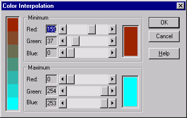
To specify a color gradient, mark all the iso values including min in the list and choose the Fill Color button to open the color gradient dialog box. You can adjust the colors for the smallest (Minimum) and the largest (Maximum) value by dragging the scroll box. The color gradient will be displayed in the left field of the dialog box. Choose OK to apply the new color gradient to the iso values in the list box.

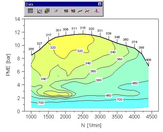
Diagram and Axes Titles

To create a title for the document, choose the Text button from the toolbar. The cursor will change to a cross with the label new. Drag a rectangle above the upper diagram to specify the size of the text box. Double-click the new text object to open the Text Object dialog box.

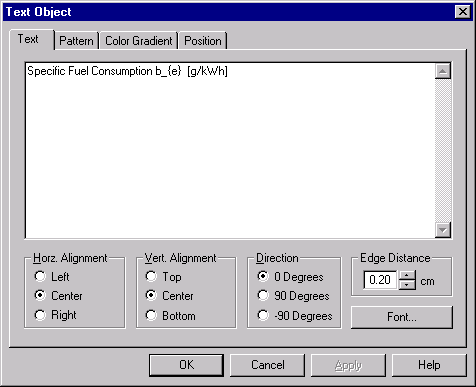
Type the following text into the edit field:

Specific Fuel Consumption b_{e}  [g/kWh]

The text object’s font and frame can be changed by selecting the appropriate button or tab in the dialog box.

If you move the cursor over the different elements of a diagram, the cursor changes to a cross with a label. For example, over the axis title, the cursor will display the text Title, over the axis labels, Label and over the diagram axis, Axis. When you double-click one of these elements you can open the dialog box to change the options.

Position the cursor on the x-axis title and open the title dialog box. Type in the following text:

Speed [rpm]

and then choose the OK button.

Editing Diagram Configuration

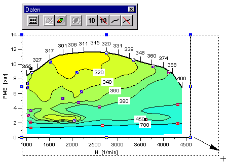
To resize a diagram, drag one of the blue handles. To move a diagram to a new position, grab the diagram between the blue handles. When the cursor is over the frame of the diagram, it will change to a cross. The size of the diagram will be displayed in the status bar in centimeters.

Importing a 2D Dataset

To import a dataset into the lower diagram, click inside the frame of the diagram with the name Diagram 2. The name of the diagram will be displayed in the combo box in the toolbar. To load a 2D dataset, choose File=>Import Data. In the Open dialog box, choose the vollast.asc file and then choose the OK button.

The file will be converted to a netCDF file and the Import dialog box will be displayed. Choose the 2D button and select N (speed) for the x-column. For the y-column, choose PME. To create the dataset, choose the Load button.

_id-1590966